Analyzing the US election using Twitter and Meta-Data in R

For my first blog post on R, I want to show how to use R to mine Twitter-data. I wanted to write this guide for several reasons. First, while there are many other guides on R-Bloggers that show similar things, they tend to focus more on setting up your Twitter account and using wordclouds. As researchers however, we are often also interested in comparing and contrasting data between groups. Meta-data can be a rich source of information for that. This approach also means that the scripts we want to write have to be more reusable in nature in order to retrieve, load, and analyze several different groups repeatedly. To this end, I will provide some simple functions built on top of other packages that enable you to download tweets from pre-specified groups of people instead of just whoever tweets on a certain topic.
Lastly, I wanted to show how analysing the Twitter meta-data in addition to the tweets themselves can lead to better behavioural insights.

This guide requires that you have a Twitter account, R(studio), and have setup a twitter-dev account with OAuth. I’ll leave the details of how to get OAuth and dev-app running here, since it explains it better than I would have been able to.

By the end of this guide you will be able to download tweets from specific users and from lists, plotting commonly used words and examining tweeting activity using meta-data. I am going to use a combination of the excellent twitteR package and httr for pulling tweets,

#Packages required:
library(twitteR)
library(ggplot2)
library(httr)
library(rjson)
library(tm)
library(gridExtra)
library(lubridate)
library(SnowballC)

If you don’t have these packages, then use

install.packages("NameOfPackage")

before running the code above. To get a feel for the commands we will pass through the code, I urge you to have a look at Twitter’s API documentation.

# Type in your app details from Twitter here:
setup_twitter_oauth(API_key, API_secret, access_token, access_secret)

A starting point: The US election

To get warmed up, let’s see what the two US presidential nominees have been talking about.
Downloading tweets from a single user is very easy, just use the

userTimeline()

function from the twitteR package.

# n specifies how many tweets you want from the user. We will use 200 in this example, but the maximum is 3200. Unfortunately you can't use the API to request tweets older than a week or two at most. This is a restriction of the Twitter Search API, and it often means you won't actually get the number of tweets you specified.  

clinton_tweets <- userTimeline(user = "@HillaryClinton", n = 200, includeRts = FALSE, retryOnRateLimit = 2000)
trump_tweets <- userTimeline(user = "@realDonaldTrump", n = 200, includeRts = FALSE, retryOnRateLimit = 2000)  

# Put the tweets downloaded into a data.frame
clinton_tweets <- twListToDF(clinton_tweets)
trump_tweets <- twListToDF(trump_tweets)

If you do not include retweets you will quite not get the amount of tweets you specified (as they are counted but not downloaded). If you want to save these tweets for a later time, then use write.csv(downloadedData, "nameCSV.csv") to write the tweets to your hard drive. Now that we have the tweets down, it is useful to remove any unneccesary fluff:

# Remove punctuation, numbers, html-links and unecessary spaces:
textScrubber <- function(dataframe) {
    
    dataframe$text <-  gsub("http\\S+\\s*", "", dataframe$text)
    dataframe$text <-  gsub("\n", " ", dataframe$text)
    dataframe$text <-  gsub("https\\w+", "", dataframe$text)
    dataframe$text <-  gsub("http\\w+", "", dataframe$text)
    dataframe$text <-  gsub("—", " ", dataframe$text)
    dataframe$text <-  gsub("&amp;", " ", dataframe$text)
    dataframe$text <-  gsub("[[:punct:]]", " ", dataframe$text)
    dataframe$text <-  gsub("[[:digit:]]", " ", dataframe$text)
    dataframe$text <-  tolower(dataframe$text)
    
    return(dataframe)
}

To run the function, type in:

clinton_tweets <- textScrubber(clinton_tweets)
trump_tweets <- textScrubber(trump_tweets)

After that, we remove all the so-called “stopwords”(words that do not add meaning to the topic), and convert the text into a Term Document Matrix. The TDM is then summed up so we get a data.frame of words arranged by how often they are used

tdmCreator <- function(dataframe, stemDoc = T, rmStopwords = T){
    
    tdm <- Corpus(VectorSource(dataframe$text))
    if (isTRUE(rmStopwords)) {
        tdm <- tm_map(tdm, removeWords, stopwords())
    }
    if (isTRUE(stemDoc)) {
        tdm <- tm_map(tdm, stemDocument)
    }
    tdm <- TermDocumentMatrix(tdm, control = list(wordLengths = c(1, Inf)))
    tdm <- rowSums(as.matrix(tdm))
    tdm <- sort(tdm, decreasing = T)
    df <- data.frame(term = names(tdm), freq = tdm)
    return(df)
}

Making a function like this is not strictly necessary, and if you want to do serious text mining (or sentiment analysis, then it is advisable to save a separate TDM for later use. For now though, having a function makes repeating the same code over and over again a little easier. The function takes two extra arguments. StemDoc asks if you want to stem the text, making the computer try to make words that are similar appear as the same. So “great” and “greater” gets treated as the same identity. rmStopwords simply removes words that are often used but don’t add any additional meaning. I have defaulted them to true in this example for both, but you can experiment with switching these on and off to see how it affects your results.
To clean the tweets, simply pass

clinton_tweets <- tdmCreator(clinton_tweets)
trump_tweets <- tdmCreator(trump_tweets)

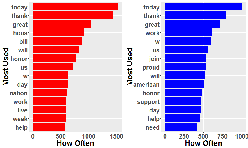
Finally we can plot each of the candidates most used words:

# Selects the 15 most used words.
trump_tweets <- trump_tweets[1:15,]
clinton_tweets <- clinton_tweets[1:15,]

# Create bar graph with appropriate colours and use coord_flip() to help the labels look nicer.
trump_plot <- ggplot(trump_tweets, aes(x = reorder(term, freq), y = freq)) +
    geom_bar(stat = "identity", fill = "red") +
    xlab("Most Used") + ylab("How Often") +
    coord_flip() + theme(text=element_text(size=25,face="bold"))

clinton_plot <- ggplot(clinton_tweets, aes(x = reorder(term, freq), y = freq)) +
    geom_bar(stat = "identity", fill = "blue") +
    xlab("Most Used") + ylab("How Often") +
    coord_flip() + theme(text=element_text(size=25,face="bold"))

# There are other ways to get these plots side-by-side, but this is easy.
grid.arrange(trump_plot, clinton_plot, ncol=2)

At the time of writing, these tweets are a little old, but they still convey a good deal of information. It is immediately obvious that both Trump and Clinton spend a great deal of time talking about Trump. Especially Hillary seems to really try to mention him as much as possible. Trump talking about himself is not really that much of a surprise…

But that’s only for two Twitter-accounts. What if we wanted to look at a selected sample or a section of a population? If you are just interested in massive, massive amounts of data, then Twitter lets you sample 1% of their tweets using a specified function. This is relatively noisy though and if you don’t know what you are looking for, then you aren’t likely to find anything either. There are other guides that show you how to do this, but I want to show instead how we can use twitter-lists to mine data from a pre-specified group/list of people instead. After you have created your list you can simply download all the latest tweets from them using a simple for loop.

Comparing groups of tweeters

To make things easier, I have made the previous step into a function built on top of twitteR::userTimeline():

# Download tweets from a group of people specified in a Twitter list.
tweetsFromList <- function (listOwner, listName, sleepTime = 7, n_tweets = 200, includeRts = F) {

api_url <- paste0("https://api.twitter.com/1.1/lists/members.json?slug=",
                  listName, "&owner_screen_name=", listOwner, "&count=5000")
# Pull out the users from the list
response <- GET(api_url, config(token=twitteR:::get_oauth_sig()))
response_data <- fromJSON(content(response, as = "text", encoding = "UTF-8"))
## If you want a list of their profile names, then remove the hastag underneath and
## add it to the return statement at the bottom (use a list).
## Useful if you need to verify identity of people.
    
#user_title <- sapply(response_text$users, function(i) i$name)
user_names <- sapply(response_data$users, function(i) i$screen_name)
tweets <- list()
## Loops over list of users, use rbind() to add them to list.
## Sleeptime ticks inbetween to avoid rate limit.
   for (user in user_names) {
    ## Download user's timeline from Twitter  
    raw_data <- userTimeline(user, n = n_tweets,
                             includeRts = includeRts,
                             retryOnRateLimit = 2000)
        if (length(raw_data) != 0L) {
            tweets <- rbind(tweets, raw_data)
        print('Sleeping to avoid rate limit')
        Sys.sleep(sleepTime);
# If a Twitter-user has no tweets, userTimeline and rbind fails. The if-else statement solves this.
        }
            else {
                next
            }
         
        }
rm(raw_data)
tweets <- twListToDF(tweets)    
return(tweets)
}

Twitter-lists are lists of Twitter members that users create on Twitter in order to filter their home feed and only recieve tweets from those members. These lists are useful for data-mining since they allow us to put people in different quasi-experimental groups that we can then compare afterwards. So all you need to do is to create separate lists of the groups of people you want to extract tweets from. If you don’t have your own lists (they are easy to make), then you can also just use someone elses list. Simply supply the function with the list owner, as well as the name of the list.
To continue our investigation into the political world, let’s compare tweets from Democrat and Republican House Representatives.

republicans <- tweetsFromList("HouseGOP", "house-republicans")
democrats <- tweetsFromList("TheDemocrats", "house-democrats")

Note that both of these commands will take some time as there will be a lot of tweets downloaded. To get an idea for how many tweets, use this formula: (number of list members * 7 sec)/60sec. There’s 261 Republicans in our list, so that means it will take a minumum of 31 minutes to download all the tweets. If you want it to go faster you can adjust the sleepTime parameter. Note however that if you set it below 5, then the Twitter API will start throttling you. Go grab a drink instead.

After that is done it is strongly advised that you save the contents to your hard drive (so you won’t have to download them all at once again). Use write.csv(nameOfFile, "nameOfCSV.csv") to save it in your working directory.

All done? Excellent, now we have a lot of data to work with. Let’s re-run the previous analysis and plot the graphs I have ommited the plotting code as it is identical to the one used above.

democrats <- read.csv("democrats.csv")
republicans <- read.csv("republicans.csv")
democrats <- textScrubber(democrats)
republicans <- textScrubber(republicans)

# Warning: this step requires a lot of working memory available. If you do not have this, add the removeSparseTerms(tdm, .97) to the tdmCreator function code (before the rowSums call)
dem <- tdmCreator(democrats)
rep <- tdmCreator(republicans)

That is certainly interesting. Turns out the House actually seems to care about the same things! Being up for re-election so much of the time seems to have a rather humbling effect.

Using meta-data to dig even deeper.

That’s all fine and good, but to really gain an understanding of their differences it is useful to look at some of the meta-data. For some reason this is rarely used in other guides on analyzing tweets, but I think they are useful to check for a couple of things:

• Do politicians have different tweeting strategies?
• Do they for example tweet at different times of day to target their preferred audience?
• Do they all carefully schedule their tweets, or can they be more impulsive (dependent on party)?

This is not an exhaustive list of topics that can be investigated, but there is a lot you can do with the meta-data that also gets downloaded. use the stror View() function to investigate the data.frame of tweets yourself and you will se that there are numerous other things apart from just the tweets that gets downloaded. Let’s start with a comparison of when democrats and republicans tweet:

democrats$group <- as.factor("dem")
republicans$group <- as.factor("rep")
# Create one large data.frame for comparison
both <- rbind(democrats, republicans)

# Use the lubridate package to make working with time easier.
both$date <- ymd_hms(both$created)
both$hour <- hour(both$date) + minute(both$date)/60
both$day <- weekdays(as.Date(both$date))
#rearrange the weekdays in chronological order
both$day <- factor(both$day, levels = c("Monday", "Tuesday", "Wednesday", "Thursday", "Friday", "Saturday", "Sunday"))
#this last re-factoring just makes the colors in the plot correct. For your own groups you want to remove the line of code underneath.
both$group <- factor(both$group, levels = c("rep", "dem"))

ggplot(both, aes(hour, colour = group)) + geom_density()
ggplot(both, aes(hour, colour = group)) + geom_density() + facet_wrap(~day, nrow = 3)

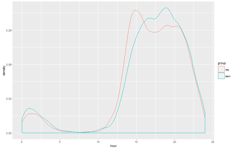
Voila; a kernel density plot showing when tweets appear. There actually seems to be a large gap in the peaks between the political representatives! Also notice that democrats are slightly more likely to stay up late at night to tweet. Maybe they are more “liberal”” with the alcohol and therefore have less impulse control? One can only imagine…

If we divide up the plot by each days we also get a lot of info:

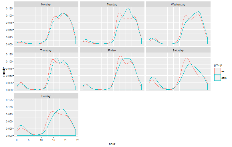
Republicans have their peak almost always at 15:00 every single day. I am not American myself so I don’t know the political system well enough, but that does seem like something a little too odd to just be a coincidence. Feel free to come with suggestions in the comments. On a more humourous note, the late-night bump for the democrats are even more pronounced during the weekend.

Who schedules the most and who tweets more on the fly?

To answer this question, we tidy up and count the different names found in the “StatusSource”-part of our data.frame. This will act as a proxy for scheduling (as this is a function limited to certain platforms):

device <- function(dataframe) {
    tot_all <- length(dataframe$statusSource)

    Web <- 100*(length(grep("Twitter Web Client", dataframe$statusSource))/tot_all)
    TweetDeck <- 100*(length(grep("TweetDeck", dataframe$statusSource))/tot_all)
    iPhone <- 100*(length(grep("Twitter for iPhone", dataframe$statusSource))/tot_all)
    iPad <- 100*(length(grep("Twitter for iPad", dataframe$statusSource))/tot_all)
    Blackberry <- 100*(length(grep("Twitter for BlackBerry", dataframe$statusSource))/tot_all)
    Tweetbot <- 100*(length(grep("Tweetbot for i", dataframe$statusSource))/tot_all)
    Hootsuite <- 100*(length(grep("Hootsuite", dataframe$statusSource))/tot_all)
    Android <- 100*(length(grep("Twitter for Android", dataframe$statusSource))/tot_all)
    Ads <- 100*(length(grep("Twitter Ads", dataframe$statusSource))/tot_all)
    M5 <- 100*(length(grep("Mobile Web (M5)", dataframe$statusSource))/tot_all)
    Mac <- 100*(length(grep("Twitter for Mac", dataframe$statusSource))/tot_all)
    Facebook <- 100*(length(grep("Facebook", dataframe$statusSource))/tot_all)
    Instagram <- 100*(length(grep("Instagram", dataframe$statusSource))/tot_all)
    IFTT <- 100*(length(grep("IFTT", dataframe$statusSource))/tot_all)
    Buffer <- 100*(length(grep("Buffer", dataframe$statusSource))/tot_all)
    CoSchedule <- 100*(length(grep("CoSchedule", dataframe$statusSource))/tot_all)
    GainApp <- 100*(length(grep("Gain App", dataframe$statusSource))/tot_all)
    MobileWeb <- 100*(length(grep("Mobile Web", dataframe$statusSource))/tot_all)
    iOS <- 100*(length(grep("iOS", dataframe$statusSource))/tot_all)
    OSX <- 100*(length(grep("OS X", dataframe$statusSource))/tot_all)
    Echofon <- 100*(length(grep("Echofon", dataframe$statusSource))/tot_all)
    Fireside <- 100*(length(grep("Fireside Publishing", dataframe$statusSource))/tot_all)
    Google <- 100*(length(grep("Google", dataframe$statusSource))/tot_all)
    MailChimp <- 100*(length(grep("MailChimp", dataframe$statusSource))/tot_all)
    TwitterForWebsites <- 100*(length(grep("Twitter for Websites", dataframe$statusSource))/tot_all)
    
    percentages <- data.frame(Web, TweetDeck, iPhone, iPad, Blackberry, Tweetbot,
               Hootsuite, Android, Ads, M5, Mac, Facebook, Instagram,
               IFTT, Buffer, CoSchedule, GainApp, MobileWeb, iOS, OSX,
               Echofon, Fireside, Google, MailChimp, TwitterForWebsites)
    return(percentages)
}

Now we can sort by most popular devices:

repDevice <- sort(device(republicans), decreasing = T)
demDevice <- sort(device(democrats), decreasing = T)
clintonDevice <- sort(device(clinton_tweets), decreasing = T)
trumpDevice <- sort(device(trump_tweets), decreasing = T)
#pick out the top 5 platforms:
repDevice[ ,1:5]
#   Web TweetDeck   iPhone Hootsuite Facebook
#50.40192  21.82417 17.07703  3.487563 1.424141
demDevice[ ,1:5]
#   Web   iPhone TweetDeck Hootsuite     iPad
#51.41274 20.81256  17.50693  2.705448 1.745152
trumpDevice[ ,1:5]
#   Android   iPhone      Web TweetDeck iPad
# 62.62626 28.28283 9.090909         0    0  
clintonDevice[ ,1:5]
#   TweetDeck    Web   iPhone iPad Blackberry
#  73.02632 21.05263 5.921053    0          0

That’s some pretty big differences there between Trump and Hillary especially. Whereas Hillary seems to use Tweetdeck the most (probably to schedule tweets), Trump seems to live and die by his two phones.This is consistent with his impulsive image.

Republicans and Democrats are more similar, especially in how no-one uses Android phones. Looks like if you’re an American representative, then you better use American products. But note how Republicans seem to use scheduling services (TweetDeck and Hootsuite) more often. This could potentially explain the 15:00 bump that we found previously.

A more thorough investigation could look at what type of platforms were most used around that time of day, but this article is already getting quite long. So I am going to stop here, and I hope you will play around with the code yourself to see what you can find. In the future I am hoping to make a post on combining different sorts of meta-data using the dplyr package to answer even more fine-grained questions.

• If you have any questions, or something isn’t working as it should, please feel free to contact me @andreasose.